Cancer Metastasis
BooLEVARD Tutorials
[Tutorial 3] Activatory perturbations of p63, p53, and miR34 dampen cancer invasiveness.
In this tutorial, we will use a Boolean model representing key molecular cascades in cancer metastasis. The tutorial showcases how activatory perturbations of two tumor suppressor (p53 and p63) and micro RNA 34 successfully dampen invasiveness and increases apoptotic cell-fate decisions. This model is available in Cell Collective (SBML) and GinSIM’s model repository (ZGINML). This model was used as a showcase in the BooLEVARD’s paper, for which a BoolNet version was generated, and therefore, we will use that version. To know how to convert Boolean models in SBML format to BoolNet format, please refer to Tutorial 2.
Cohen DPA, Martignetti L, Robine S, Barillot E, Zinovyev A, et al. (2015). Mathematical Modelling of Molecular Pathways Enabling Tumour Cell Invasion and Migration. PLOS Computational Biology 11(11): e1004571. https://doi.org/10.1371/journal.pcbi.1004571
[1]:
import boolevard as blv
import pandas as pd
import numpy as np
import matplotlib.pyplot as plt
/home/marco/.local/lib/python3.11/site-packages/pandas/core/arrays/masked.py:60: UserWarning: Pandas requires version '1.3.6' or newer of 'bottleneck' (version '1.3.5' currently installed).
  from pandas.core import (
/home/marco/.local/lib/python3.11/site-packages/matplotlib/projections/__init__.py:63: UserWarning: Unable to import Axes3D. This may be due to multiple versions of Matplotlib being installed (e.g. as a system package and as a pip package). As a result, the 3D projection is not available.
  warnings.warn("Unable to import Axes3D. This may be due to multiple versions of "
We will load the model and set up the Apoptosis and Invasion phenotype nodes as read outs. In addition, we will define a set of perturbations to perform (inhibition of AKT1 and AKT2, and activation of p53), in order to study their inpact in the apoptotic and invasive fates. Let’s first load the model and retrieve some basic information:
[37]:
model = blv.Load("resources/Cohen_2015.bnet") # Load the model (BoolNet format)
model.Info.columns = list(range(len(model.Info.columns)-2)) + ["DNF", "NDNF"] # Let's reset the stable states so that they start from 0
phenotypes = ["Apoptosis", "Invasion"] # Set node(s) to check
perturbations = ["p63%ACT", "p53%ACT", "miR34%ACT"] # Set list of perturbations to apply
print(f"Number of nodes: {len(model.Nodes)}")
print(f"Number of inputs: {len(model.Info.index[model.Info.index == model.Info['DNF'].apply(str)])}, ({', '.join(list((model.Info.index[model.Info.index == model.Info['DNF'].apply(str)])))})")
print(f"Number of stable states: {len(model.Info.columns)-2}")
Number of nodes: 33
Number of inputs: 2, (ECMicroenv, DNAdamage)
Number of stable states: 9
[38]:
model.Info
[38]:
| 0 | 1 | 2 | 3 | 4 | 5 | 6 | 7 | 8 | DNF | NDNF | |
|---|---|---|---|---|---|---|---|---|---|---|---|
| TGFbeta_e | 0 | 0 | 0 | 0 | 0 | 1 | 1 | 1 | 1 | ECMicroenv | ~ECMicroenv |
| TGFbeta_i | 0 | 0 | 0 | 0 | 0 | 0 | 0 | 1 | 1 | And(~CTNNB1, NICD) | Or(CTNNB1, ~NICD) |
| TGFbeta | 0 | 0 | 0 | 0 | 0 | 1 | 1 | 1 | 1 | Or(TGFbeta_e, TGFbeta_i) | And(~TGFbeta_e, ~TGFbeta_i) |
| ECMicroenv | 0 | 0 | 0 | 0 | 0 | 1 | 1 | 1 | 1 | ECMicroenv | ~ECMicroenv |
| GF | 0 | 0 | 0 | 1 | 1 | 0 | 0 | 1 | 1 | Or(And(~CDH1, CDH2), And(~CDH1, GF)) | Or(CDH1, And(~CDH2, ~GF)) |
| CDH1 | 1 | 1 | 1 | 0 | 0 | 1 | 1 | 0 | 0 | And(~AKT2, ~SNAI1, ~SNAI2, ~TWIST1, ~ZEB1, ~ZEB2) | Or(AKT2, SNAI1, SNAI2, TWIST1, ZEB1, ZEB2) |
| ERK | 0 | 0 | 0 | 1 | 1 | 0 | 0 | 1 | 1 | Or(And(~AKT1, CDH2), And(~AKT1, GF), And(~AKT1... | Or(AKT1, And(~CDH2, ~GF, ~NICD, ~SMAD)) |
| EMT | 0 | 0 | 0 | 1 | 1 | 0 | 0 | 1 | 1 | And(~CDH1, CDH2) | Or(CDH1, ~CDH2) |
| CDH2 | 0 | 0 | 0 | 1 | 1 | 0 | 0 | 1 | 1 | TWIST1 | ~TWIST1 |
| VIM | 0 | 0 | 0 | 1 | 1 | 0 | 0 | 1 | 1 | Or(CTNNB1, ZEB2) | And(~CTNNB1, ~ZEB2) |
| SNAI1 | 0 | 0 | 0 | 1 | 1 | 0 | 0 | 1 | 1 | Or(And(~CTNNB1, NICD, ~miR203, ~miR34, ~p53), ... | Or(CTNNB1, miR203, miR34, p53, And(~NICD, ~TWI... |
| ZEB2 | 0 | 0 | 0 | 1 | 1 | 0 | 0 | 1 | 1 | Or(And(NICD, ~miR200, ~miR203), And(SNAI1, ~mi... | Or(miR200, miR203, And(~NICD, ~SNAI1, ~SNAI2),... |
| SNAI2 | 0 | 0 | 0 | 1 | 1 | 0 | 0 | 1 | 1 | Or(And(CTNNB1, ~miR200, ~miR203, ~p53), And(NI... | Or(miR200, miR203, p53, And(~CTNNB1, ~NICD, ~T... |
| ZEB1 | 0 | 0 | 0 | 1 | 1 | 0 | 0 | 1 | 1 | Or(And(CTNNB1, ~miR200), And(NICD, ~miR200), A... | Or(miR200, And(~CTNNB1, ~NICD, ~SNAI1, ~SNAI2)... |
| TWIST1 | 0 | 0 | 0 | 1 | 1 | 0 | 0 | 1 | 1 | Or(CTNNB1, NICD, SNAI1) | And(~CTNNB1, ~NICD, ~SNAI1) |
| NICD | 0 | 0 | 0 | 0 | 0 | 0 | 0 | 1 | 1 | And(ECMicroenv, ~miR200, ~miR34, ~p53, ~p63, ~... | Or(~ECMicroenv, miR200, miR34, p53, p63, p73) |
| DKK1 | 0 | 0 | 0 | 0 | 0 | 0 | 0 | 1 | 1 | Or(CTNNB1, NICD) | And(~CTNNB1, ~NICD) |
| SMAD | 0 | 0 | 0 | 0 | 0 | 0 | 0 | 1 | 1 | And(TGFbeta, ~miR200, ~miR203) | Or(~TGFbeta, miR200, miR203) |
| CTNNB1 | 0 | 0 | 0 | 0 | 0 | 0 | 0 | 0 | 0 | And(~AKT1, ~CDH1, ~CDH2, ~DKK1, ~miR200, ~miR3... | Or(AKT1, CDH1, CDH2, DKK1, miR200, miR34, p53,... |
| AKT2 | 0 | 0 | 0 | 1 | 1 | 0 | 0 | 1 | 1 | Or(And(CDH2, TWIST1, ~miR203, ~miR34, ~p53), A... | Or(~TWIST1, miR203, miR34, p53, And(~CDH2, ~GF... |
| AKT1 | 0 | 0 | 0 | 0 | 0 | 0 | 0 | 0 | 0 | Or(And(~CDH1, CDH2, CTNNB1, ~miR34, ~p53), And... | Or(CDH1, ~CTNNB1, miR34, p53, And(~CDH2, ~GF, ... |
| miR203 | 0 | 0 | 1 | 0 | 0 | 0 | 1 | 0 | 0 | And(~SNAI1, ~ZEB1, ~ZEB2, p53) | Or(SNAI1, ZEB1, ZEB2, ~p53) |
| miR200 | 0 | 1 | 1 | 0 | 0 | 1 | 1 | 0 | 0 | Or(And(~AKT2, ~SNAI1, ~SNAI2, ~ZEB1, ~ZEB2, p5... | Or(AKT2, SNAI1, SNAI2, ZEB1, ZEB2, And(~p53, ~... |
| miR34 | 0 | 0 | 0 | 0 | 0 | 0 | 0 | 0 | 0 | Or(And(~AKT1, AKT2, ~SNAI1, ~ZEB1, ~ZEB2, p53,... | Or(AKT1, ~AKT2, SNAI1, ZEB1, ZEB2, p63, And(~p... |
| Migration | 0 | 0 | 0 | 0 | 0 | 0 | 0 | 1 | 1 | And(~AKT1, AKT2, EMT, ERK, Invasion, VIM, ~miR... | Or(AKT1, ~AKT2, ~EMT, ~ERK, ~Invasion, ~VIM, m... |
| Invasion | 0 | 0 | 0 | 0 | 0 | 0 | 0 | 1 | 1 | Or(CTNNB1, And(CDH2, SMAD)) | Or(And(~CDH2, ~CTNNB1), And(~CTNNB1, ~SMAD)) |
| CellCycleArrest | 0 | 1 | 1 | 1 | 1 | 1 | 1 | 1 | 1 | Or(And(~AKT1, ZEB2), And(~AKT1, miR200), And(~... | Or(AKT1, And(~ZEB2, ~miR200, ~miR203, ~miR34, ... |
| p21 | 0 | 1 | 1 | 0 | 0 | 1 | 1 | 0 | 0 | Or(And(~AKT1, AKT2, ~ERK), And(~AKT1, ~ERK, NI... | Or(AKT1, ERK, And(~AKT2, ~NICD, ~p53, ~p63, ~p... |
| p73 | 0 | 1 | 0 | 0 | 0 | 1 | 0 | 0 | 0 | And(~AKT1, ~AKT2, DNAdamage, ~ZEB1, ~p53) | Or(AKT1, AKT2, ~DNAdamage, ZEB1, p53) |
| p53 | 0 | 0 | 1 | 0 | 0 | 0 | 1 | 0 | 0 | Or(And(~AKT1, ~AKT2, CTNNB1, ~SNAI2, ~p73), An... | Or(AKT1, AKT2, SNAI2, p73, And(~CTNNB1, ~DNAda... |
| Apoptosis | 0 | 1 | 1 | 0 | 0 | 1 | 1 | 0 | 0 | Or(And(~AKT1, ~ERK, ~ZEB2, miR200), And(~AKT1,... | Or(AKT1, ERK, ZEB2, And(~miR200, ~miR34, ~p53,... |
| p63 | 0 | 1 | 0 | 0 | 0 | 1 | 0 | 0 | 0 | And(~AKT1, ~AKT2, DNAdamage, ~NICD, ~miR203, ~... | Or(AKT1, AKT2, ~DNAdamage, NICD, miR203, p53) |
| DNAdamage | 0 | 1 | 1 | 0 | 1 | 1 | 1 | 0 | 1 | DNAdamage | ~DNAdamage |
The model reaches a total of 9 stable states upon any combination of the local states ECMicroenv and DNAdamage input nodes. We can observe that Apoptosis is active in 4 states (1, 2, 5, 6), whereas Invasion is active in two (7, 8).
Apoptosis: reached upon DNAdamage, DNAdamage and ECMicroenv.
Invasion: reached upon ECMicroenv, DNAdamage and ECMicroenv.
Let’s now count the paths toward these phenotype nodes across every stable state:
[4]:
paths = model.CountPaths(phenotypes, ss_wise = True) # Count the number of paths leading to the Apoptosis and Invasion nodes
Evaluating Stable State: 0
Apoptosis: -355, 1.0629494984944662e-05 minutes.
Invasion: -96, 2.3802121480305988e-06 minutes.
Evaluating Stable State: 1
Apoptosis: 650803, 0.03362019062042236 minutes.
Invasion: -79488, 0.004182140032450358 minutes.
Evaluating Stable State: 2
Apoptosis: 547393, 0.031016747156778973 minutes.
Invasion: -137450, 0.007069091002146403 minutes.
Evaluating Stable State: 3
Apoptosis: -92533, 0.005101394653320312 minutes.
Invasion: -2867, 0.0001383662223815918 minutes.
Evaluating Stable State: 4
Apoptosis: -2371, 0.0008930842081705729 minutes.
Invasion: -213, 4.831155141194661e-05 minutes.
Evaluating Stable State: 5
Apoptosis: 69198, 0.007056013743082682 minutes.
Invasion: -7297, 0.0008472879727681478 minutes.
Evaluating Stable State: 6
Apoptosis: 47620, 0.008798758188883463 minutes.
Invasion: -10026, 0.001911294460296631 minutes.
Evaluating Stable State: 7
Apoptosis: -4106274, 0.27379823525746666 minutes.
Invasion: 554895, 0.04231379429499308 minutes.
Evaluating Stable State: 8
Apoptosis: -1376996, 0.17505908807118734 minutes.
Invasion: 179328, 0.025075976053873697 minutes.
[39]:
paths_sum = pd.DataFrame(paths)
paths_sum.columns = phenotypes
paths_sum
[39]:
| Apoptosis | Invasion | |
|---|---|---|
| 0 | -355 | -96 |
| 1 | 650803 | -79488 |
| 2 | 547393 | -137450 |
| 3 | -92533 | -2867 |
| 4 | -2371 | -213 |
| 5 | 69198 | -7297 |
| 6 | 47620 | -10026 |
| 7 | -4106274 | 554895 |
| 8 | -1376996 | 179328 |
We observe that stable states triggering Apoptosis can be divided into two groups based on the number of paths activating this phenotype:
Higher Apoptosis (HiA): stable state 1 (DNAdamage: ON, ECMicroenv: OFF) and stable state 2 (DNAdamage: ON, ECMicroenv: OFF)
Lower Apoptosis (LoA): stable state 5 (DNAdamage: ON, ECMicroenv: ON) and stable state 6 (DNAdamage: ON, ECMicroenv: ON)
The HiA states have around 10 times more paths inhibiting apoptosis than the LoA ones.
Regarding the stable states triggering Invasion, we have one with around 3 times more paths than the other:
Higher Invasion (HiI): stable state 7 (DNAdamage: OFF, ECMicroenv: ON)
Lower Invasion (LoI): stable state 8 (DNAdamage: ON, ECMicroenv: ON)
We observe that DNAdamage negatively impacts the ECMicroenv-triggered invassive fate, and that ECMicroenv negatively impacts the DNAdamage-triggered apoptotic fate.
Let’s now perform the perturbations and count the paths triggering the states of this phenotype nodes:
[43]:
pert_models = {
    "Unperturbed": model,
    "p63a": model.Pert(perturbations[0]),
    "p53a": model.Pert(perturbations[1]),
    "miR34a": model.Pert(perturbations[2])
}

pert_paths = {}
for key in pert_models:
    pert_models[key].Info.columns = list(range(len(pert_models[key].Info.columns)-2)) + ["DNF", "NDNF"]
    pert_models[key].Info = pert_models[key].Info.loc[:, ~((pert_models[key].Info.loc["ECMicroenv"] == 0) & (pert_models[key].Info.loc["DNAdamage"] == 0))]
    pert_paths[key] = pd.DataFrame(pert_models[key].CountPaths(phenotypes, ss_wise=True))
    pert_paths[key].columns = phenotypes
    pert_paths[key].index = pert_models[key].Info.columns[:-2]
Evaluating Stable State: 1
Apoptosis: 650803, 0.03550153175989787 minutes.
Invasion: -79488, 0.004427965482076009 minutes.
Evaluating Stable State: 2
Apoptosis: 547393, 0.031353513399759926 minutes.
Invasion: -137450, 0.007886393864949545 minutes.
Evaluating Stable State: 4
Apoptosis: -2371, 0.0009159564971923829 minutes.
Invasion: -213, 4.942417144775391e-05 minutes.
Evaluating Stable State: 5
Apoptosis: 69198, 0.007487761974334717 minutes.
Invasion: -7297, 0.0009128570556640625 minutes.
Evaluating Stable State: 6
Apoptosis: 47620, 0.009185870488484701 minutes.
Invasion: -10026, 0.002027567227681478 minutes.
Evaluating Stable State: 7
Apoptosis: -4106274, 0.29480555057525637 minutes.
Invasion: 554895, 0.04455423355102539 minutes.
Evaluating Stable State: 8
Apoptosis: -1376996, 0.18616377115249633 minutes.
Invasion: 179328, 0.026827104886372886 minutes.
Evaluating Stable State: 1
Apoptosis: 726108, 0.03727216323216756 minutes.
Invasion: -85524, 0.004598780473073324 minutes.
Evaluating Stable State: 2
Apoptosis: 2597481, 0.09866807063420614 minutes.
Invasion: -418316, 0.015083523591359456 minutes.
Evaluating Stable State: 4
Apoptosis: -8087, 0.0008593916893005372 minutes.
Invasion: -157, 3.064473470052083e-05 minutes.
Evaluating Stable State: 5
Apoptosis: 4519, 0.0001856406529744466 minutes.
Invasion: -696, 3.170569737752278e-05 minutes.
Evaluating Stable State: 6
Apoptosis: 98526, 0.007704083124796549 minutes.
Invasion: -9770, 0.0009197592735290527 minutes.
Evaluating Stable State: 7
Apoptosis: 505441, 0.02979077895482381 minutes.
Invasion: -70079, 0.004510140419006348 minutes.
Evaluating Stable State: 8
Apoptosis: -76913, 0.003245238463083903 minutes.
Invasion: 13556, 0.0005586822827657064 minutes.
Evaluating Stable State: 9
Apoptosis: -16942, 0.0015027244885762532 minutes.
Invasion: 3336, 0.00028112332026163734 minutes.
Evaluating Stable State: 1
Apoptosis: 640545, 0.03310054143269857 minutes.
Invasion: -153171, 0.007697677612304688 minutes.
Evaluating Stable State: 2
Apoptosis: 47620, 0.001430976390838623 minutes.
Invasion: -10026, 0.00030887921651204426 minutes.
Evaluating Stable State: 3
Apoptosis: 95238, 0.009834237893422445 minutes.
Invasion: -20052, 0.00214764674504598 minutes.
Evaluating Stable State: 0
Apoptosis: 1998981, 0.06153324047724406 minutes.
Invasion: -194425, 0.00604479710261027 minutes.
Evaluating Stable State: 2
Apoptosis: 3493902, 0.11173041661580403 minutes.
Invasion: -577853, 0.017530858516693115 minutes.
Evaluating Stable State: 3
Apoptosis: 497384, 0.016261287530263267 minutes.
Invasion: -45067, 0.0014878908793131511 minutes.
Evaluating Stable State: 4
Apoptosis: 544103, 0.019650065898895265 minutes.
Invasion: -82159, 0.0029144962628682453 minutes.
Evaluating Stable State: 5
Apoptosis: 895925, 0.03503890832265218 minutes.
Invasion: -137210, 0.005308918158213298 minutes.
Now that we have counted the paths toward Apoptosis and Invasion phenotype nodes for the three perturbations, let’s plot the results:
[45]:
# Define a function to generate a bar plot with BooLEVARD's results for the stable states
def SSbars(data, sizex = 3, sizey = 2.5, labs = ("Invasion", "Apoptosis"), ax = None):
    def log_signed(x, base = 2):
        return np.sign(x) * np.log1p(np.abs(x))/np.log(base)
    states = data.index.astype(str).tolist()
    inv = log_signed(data["Invasion"].values, base = 2)
    apo = log_signed(data["Apoptosis"].values, base = 2)
    n = len(states)
    x_inv = np.arange(n)
    x_apo = x_inv + n + 0.5
    def col(v): return "#FC766A" if v > 0 else "#5B84B1"
    cols_inv = [col(v) for v in inv]
    cols_apo = [col(v) for v in apo]
    if ax is None:
        fig, ax = plt.subplots(figsize = (sizex, sizey))
    ax.bar(x_inv, inv, color = cols_inv, edgecolor = "white")
    ax.bar(x_apo, apo, color = cols_apo, edgecolor = "white")
    ax.axhline(0, color = "black", linestyle = "--", linewidth = 0.7)
    y_max = max(inv.max(), apo.max())
    y_min = min(inv.min(), apo.min())
    sep = y_max * 1.1
    ax.hlines(sep, x_inv[0]-0.5, x_inv[-1]+0.5, color = "black", linewidth = 0.7); ax.hlines(sep, x_apo[0]-0.5, x_apo[-1]+0.5, color = "black", linewidth = 0.7)
    ax.set_xticks(list(x_inv) + list(x_apo))
    ax.set_xticklabels(states*2, rotation = 30, ha = "right", fontsize = 7)
    ax.set_xlim(-0.5, x_apo[-1]+0.5); ax.set_ylim(y_min*1.2, y_max*1.3)
    ax.text((x_inv[0]+x_inv[-1])/2, sep*1.02, labs[0], ha="center", fontsize=9)
    ax.text((x_apo[0]+x_apo[-1])/2, sep*1.02, labs[1], ha="center", fontsize=9)
    title = getattr(data, "name", "")
    ax.set_title(title, fontweight = "bold", fontsize = 12)
    ax.set_ylabel("Path count (signed-log₂)", fontsize = 10); ax.set_xlabel("Stable States")
    plt.tight_layout()
    return ax

# Plot the results
fig, ax = plt.subplots(1, 4, figsize = (12, 3), sharey = True)
for ax, key in zip(ax, ["Unperturbed", "p63a", "p53a", "miR34a"]):
    df = pert_paths[key]
    df.name = key
    SSbars(df, sizex = 3, sizey = 3, labs = ("Invasion", "Apoptosis"), ax = ax)
plt.show()
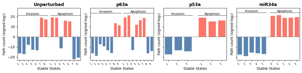
Figure 1: Barplots showing the signed-log-scaled path count score leading to the local states of Invasion and Apoptosis phenotype nodes. Each plot represents a perturbation, and bars delimited by Invasion and Apoptosis show the path count scores resulting in the inactivation (blue) or activation (red) of the Invasion and Apoptosis phenotype nodes.
p63 activatory perturbation
We can observe that upon activatory perturbation of p63, the local states of Invasion and Apoptosis are identical as in the perturbed configuration, except for an extra stable state. We still observe that there are two invasive stable states, but the paths leading to Invasion activation are substantially reduced upon p63 activatory perturbation:
[47]:
sum_upt = pd.concat([pert_models["Unperturbed"].Info.loc[["ECMicroenv", "DNAdamage"], ~pert_models["Unperturbed"].Info.columns.isin(["DNF", "NDNF"])],pert_paths["Unperturbed"].T]); sum_upt.columns.name = "Unperturbed"
sum_p63a = pd.concat([pert_models["p63a"].Info.loc[["ECMicroenv", "DNAdamage"], ~pert_models["p63a"].Info.columns.isin(["DNF", "NDNF"])],pert_paths["p63a"].T]); sum_p63a.columns.name = "p63a"
display(sum_upt); sum_p63a
| Unperturbed | 1 | 2 | 4 | 5 | 6 | 7 | 8 |
|---|---|---|---|---|---|---|---|
| ECMicroenv | 0 | 0 | 0 | 1 | 1 | 1 | 1 |
| DNAdamage | 1 | 1 | 1 | 1 | 1 | 0 | 1 |
| Apoptosis | 650803 | 547393 | -2371 | 69198 | 47620 | -4106274 | -1376996 |
| Invasion | -79488 | -137450 | -213 | -7297 | -10026 | 554895 | 179328 |
[47]:
| p63a | 1 | 2 | 4 | 5 | 6 | 7 | 8 | 9 |
|---|---|---|---|---|---|---|---|---|
| ECMicroenv | 0 | 0 | 0 | 1 | 1 | 1 | 1 | 1 |
| DNAdamage | 1 | 1 | 1 | 0 | 1 | 1 | 0 | 1 |
| Apoptosis | 726108 | 2597481 | -8087 | 4519 | 98526 | 505441 | -76913 | -16942 |
| Invasion | -85524 | -418316 | -157 | -696 | -9770 | -70079 | 13556 | 3336 |
The high apoptosis (HiA) states (1 and 2) from the Unperturbed model correspond to stable states 1 and 2 in the p63a model. These show an overall increase in apoptotic signaling under the p63a perturbation.
The low apoptosis (LoA) states (5 and 6) from the Unperturbed model match stable states 6 and 7 in the p63a model. These states also exhibit an elevated apoptotic response following p63a perturbation.
The high and low invasion (HiI and LoI) states (7 and 8, respectively) in the Unperturbed model correspond to stable states 8 and 9 in the p63a model. In this case, a marked reduction in invasive potential is observed under p63a conditions.
p53 activatory perturbation
In this case, activatory perturbation of p53 blocked the reachability of any invasive states:
[49]:
sum_p53a = pd.concat([pert_models["p53a"].Info.loc[["ECMicroenv", "DNAdamage"], ~pert_models["p53a"].Info.columns.isin(["DNF", "NDNF"])],pert_paths["p53a"].T]); sum_p53a.columns.name = "p53a"
display(sum_upt); sum_p53a
| Unperturbed | 1 | 2 | 4 | 5 | 6 | 7 | 8 |
|---|---|---|---|---|---|---|---|
| ECMicroenv | 0 | 0 | 0 | 1 | 1 | 1 | 1 |
| DNAdamage | 1 | 1 | 1 | 1 | 1 | 0 | 1 |
| Apoptosis | 650803 | 547393 | -2371 | 69198 | 47620 | -4106274 | -1376996 |
| Invasion | -79488 | -137450 | -213 | -7297 | -10026 | 554895 | 179328 |
[49]:
| p53a | 1 | 2 | 3 |
|---|---|---|---|
| ECMicroenv | 0 | 1 | 1 |
| DNAdamage | 1 | 0 | 1 |
| Apoptosis | 640545 | 47620 | 95238 |
| Invasion | -153171 | -10026 | -20052 |
The high apoptosis (HiA) states (1 and 2) in the Unperturbed model converge into a single stable state (1) in the p53a model, preserving a similar apoptotic profile.
The low apoptosis (LoA) states (5 and 6) and the high invasion (HiI) state 8 from the Unperturbed model merge into a unified pro-apoptotic and anti-invasive state (3) in the p53a model, exhibiting both increased apoptosis and reduced invasion compared to their original forms.
The remaining LoI state (7) transitions into stable state 2 in the p53a model, also showing a shift toward higher apoptosis and reduced invasive capacity.
miR34 activatory perturbation
In this case, we can see a similar trend as in the p53a, with overall even higher apoptosis and lower invasion:
[50]:
sum_miR34a = pd.concat([pert_models["miR34a"].Info.loc[["ECMicroenv", "DNAdamage"], ~pert_models["miR34a"].Info.columns.isin(["DNF", "NDNF"])],pert_paths["miR34a"].T]); sum_p53a.columns.name = "miR34a"
display(sum_upt); sum_miR34a
| Unperturbed | 1 | 2 | 4 | 5 | 6 | 7 | 8 |
|---|---|---|---|---|---|---|---|
| ECMicroenv | 0 | 0 | 0 | 1 | 1 | 1 | 1 |
| DNAdamage | 1 | 1 | 1 | 1 | 1 | 0 | 1 |
| Apoptosis | 650803 | 547393 | -2371 | 69198 | 47620 | -4106274 | -1376996 |
| Invasion | -79488 | -137450 | -213 | -7297 | -10026 | 554895 | 179328 |
[50]:
| 0 | 2 | 3 | 4 | 5 | |
|---|---|---|---|---|---|
| ECMicroenv | 0 | 0 | 1 | 1 | 1 |
| DNAdamage | 1 | 1 | 1 | 0 | 1 |
| Apoptosis | 1998981 | 3493902 | 497384 | 544103 | 895925 |
| Invasion | -194425 | -577853 | -45067 | -82159 | -137210 |
The high apoptosis (HiA) states (1 and 2) in the Unperturbed model are equivalent to stable states 0 and 2 in the p63a model, with overall more apoptotic and less invasive fates.
The low apoptosis (LoA) states (5 and 6) and the high invasion (HiA) state 8 from the Unperturbed model have also collapsed into two pro-apoptotic and anti-invasive states (3 and 5) with overall increased apoptosis and decreased invasiveness.
The remaining LoI state (7) transitions into stable state 4 in the miR34a model, also showing a shift toward higher apoptosis and reduced invasive capacity.